CycleGAN: Unpaired Image-to-Image Translation (Part 3)

---

Table of Contents

---

CycleGAN: Unpaired Image-to-Image Translation (Part 3)

In this tutorial, we will dive deeper into the training process of our unpaired image-to-image translation model. Specifically, we will train our CycleGAN model using Keras and TensorFlow and also learn how we can use it to perform unpaired image translation on novel unseen images.

This lesson is the last in a 3-part series on GANs 301:

1. CycleGAN: Unpaired Image-to-Image Translation (Part 1)
2. CycleGAN: Unpaired Image-to-Image Translation (Part 2)
3. CycleGAN: Unpaired Image-to-Image Translation (Part 3) (this tutorial)

To learn to train and use the CycleGAN model in real-time, just keep reading.

---

CycleGAN: Unpaired Image-to-Image Translation (Part 3)

In the first tutorial of this series on unpaired image-to-image translation, we introduced the CycleGAN model. We also discussed the formulation and principles that allow it to perform image-to-image translation from unpaired data. Furthermore, in the previous tutorial of this series, we discussed the Apples2Oranges Dataset and implemented the CycleGAN architecture from scratch in Keras and TensorFlow.

In this tutorial, we will continue this discussion and discuss in detail the training process of our CycleGAN model. Specifically, we will develop our data pipeline, implement the loss functions discussed in Part 1 and write our own code to train the CycleGAN model end-to-end using Keras and TensorFlow. We will also see how we can use our trained CycleGAN model to perform inference and translate images in real time.

---

Configuring Your Development Environment

To follow this guide, you need to have the TensorFlow library installed on your system.

Luckily, TensorFlow is pip-installable:

$ pip install tensorflow

---

Need Help Configuring Your Development Environment?

All that said, are you:

• Short on time?
• Learning on your employer’s administratively locked system?
• Wanting to skip the hassle of fighting with the command line, package managers, and virtual environments?
• Ready to run the code now on your Windows, macOS, or Linux system?

Then join PyImageSearch University today!

Gain access to Jupyter Notebooks for this tutorial and other PyImageSearch guides pre-configured to run on Google Colab’s ecosystem right in your web browser! No installation required.

And best of all, these Jupyter Notebooks will run on Windows, macOS, and Linux!

---

Project Structure

We first need to review our project directory structure.

Start by accessing this tutorial’s “Downloads” section to retrieve the source code and example images.

From there, take a look at the directory structure:

├── inference.py
├── outputs
│   ├── images
│   └── models
├── pyimagesearch
│   ├── CycleGANTraining.py
│   ├── __init__.py
│   ├── config.py
│   ├── data_preprocess.py
│   ├── model.py
│   └── train_monitor.py
└── train.py

In the previous tutorial of this series, we discussed the function of each file in our project directory. Furthermore, we discussed the config file details, the model architecture implementation (i.e., the model.py file), and the data preprocess procedure (i.e., the data_preprocess.py file).

In this part, we will discuss the training process of our image translation model. Specifically, we will discuss the CycleGANTraining.py and train.py files along with the implementation of the training callback, which will allow us to monitor the training process (i.e., the train_monitor.py file). Furthermore, we will also look into the inference stage of our trained CycleGAN model and discuss in detail the inference.py file.

---

Implementing CycleGAN Training

We start by implementing the CycleGANTraining class, which implements the training procedure of our CycleGAN model. With the help of this class, we implement the loss functions which we need to train our model, define one training iteration and call the optimizers to update our parameters after backpropagation.

So, let us open the CycleGANTraining.py file and discuss the code line by line to understand the training procedure better.

# import the necessary packages
from tensorflow.keras import Model
import tensorflow as tf

class CycleGANTraining(Model):
    def __init__(self, generatorG, discriminatorX, generatorF, 
        discriminatorY, **kwargs):
        super().__init__(**kwargs)
        # initialize the generators and discriminators
        self.generatorG = generatorG
        self.discriminatorX = discriminatorX
        self.generatorF = generatorF
        self.discriminatorY = discriminatorY

    def compile(self, gOptimizerG, dOptimizerX, gOptimizerF, 
        dOptimizerY, bceLoss):
        super().compile()
        # initialize the optimizers for the generator 
        # and discriminator
        self.gOptimizerG = gOptimizerG
        self.dOptimizerX = dOptimizerX
        
        self.gOptimizerF = gOptimizerF
        self.dOptimizerY = dOptimizerY

        # initialize the loss functions
        self.bceLoss = bceLoss

    def train_step(self, images):
        # grab the input images and target images
        (inputImage, targetImage) = images
    
        # initialize gradient tapes for both generator and discriminator
        with  tf.GradientTape() as genG_tape, tf.GradientTape() as discY_tape, tf.GradientTape() as genF_tape, tf.GradientTape() as discX_tape:
            # generate fake target images and cycle input images
            genImagesY = self.generatorG(inputImage, training=True)
            cycledImageX = self.generatorF(genImagesY, training=True)

            # generate fake input images and cycle-real target images
            genImagesX = self.generatorF(targetImage, training=True)
            cycledImageY = self.generatorG(genImagesX, training=True)

            # identity mapping
            samegenX = self.generatorF(inputImage, training=True)
            samegenY = self.generatorG(targetImage, training=True)

            # discriminator output for real target images
            discRealOutputY = self.discriminatorY([targetImage],
                training=True
            )

            # discriminator output for fake target images
            discFakeOutputY = self.discriminatorY([genImagesY], 
                training=True
            )

            # discriminator output for real input images
            discRealOutputX = self.discriminatorX([inputImage],
                training=True
            )

            # discriminator output for fake input images
            discFakeOutputX = self.discriminatorX([genImagesX], 
                training=True
            )

            # calculate cycle loss
            lossA = 10 * (tf.reduce_mean(tf.abs(targetImage - cycledImageY)))   
            lossB = 10 * (tf.reduce_mean(tf.abs(inputImage - cycledImageX)))
            totalCycleLoss = lossA + lossB 

            # calculate identity mapping
            idenityLossG = 10 * 0.5 * (tf.reduce_mean(tf.abs(targetImage - samegenY)))
            identityLossF = 10 * 0.5 * (tf.reduce_mean(tf.abs(inputImage - samegenX)))

            # calculate generator loss 
            ganLossG = self.bceLoss(tf.ones_like(discFakeOutputY), discFakeOutputY)
            ganLossF = self.bceLoss(tf.ones_like(discFakeOutputX), discFakeOutputX)

            # calculate all discriminator losses
            realDiscLossY = self.bceLoss(tf.ones_like(discRealOutputY),
                discRealOutputY)
            fakeDiscLossY = self.bceLoss(tf.zeros_like(discFakeOutputY),
                discFakeOutputY)    
            realDiscLossX = self.bceLoss(tf.ones_like(discRealOutputX),
                discRealOutputX)
            fakeDiscLossX = self.bceLoss(tf.zeros_like(discFakeOutputX),
                discFakeOutputX)

            # calculate total discriminator loss
            totalDiscLossY = 0.5*( realDiscLossY + fakeDiscLossY)
            totalDiscLossX = 0.5*( realDiscLossX + fakeDiscLossX)

            # calculate total generator loss
            totalGenLossG = ganLossG + totalCycleLoss + idenityLossG
            totalGenLossF = ganLossF + totalCycleLoss + identityLossF

        # calculate the generator and discriminator gradients
        generatorGradientsG = genG_tape.gradient(totalGenLossG, 
            self.generatorG.trainable_variables)
        generatorGradientsF = genF_tape.gradient(totalGenLossF, 
            self.generatorF.trainable_variables)
        discriminatorXGradients = discX_tape.gradient(totalDiscLossX, 
            self.discriminatorX.trainable_variables)
        discriminatorYGradients = discY_tape.gradient(totalDiscLossY, 
            self.discriminatorY.trainable_variables)

        # apply the gradients to both generators and discriminators
        self.gOptimizerG.apply_gradients(zip(generatorGradientsG,
            self.generatorG.trainable_variables))
        self.gOptimizerF.apply_gradients(zip(generatorGradientsF,
            self.generatorF.trainable_variables))
        self.dOptimizerX.apply_gradients(zip(discriminatorXGradients,
            self.discriminatorX.trainable_variables))
        self.dOptimizerY.apply_gradients(zip(discriminatorYGradients,
            self.discriminatorY.trainable_variables))

        # return the generator and discriminator losses
        return {"dLossX_input": totalDiscLossX, "gLossG": ganLossG+totalCycleLoss,
            "dLossY_output": totalDiscLossY, "gLossF": ganLossF+totalCycleLoss}

Let us review the pipeline of our CycleGAN model, which we discussed in detail in Part 1 of this series. We have 2 Generators (G and F) and 2 Discriminators (X and Y), which allow us to perform image-to-image translation between the apples and oranges domains without paired images.

Generator G takes images from one domain (say, apples) and translates them to images of the other domain (say, oranges), as discussed in Part 1 of this series. Furthermore, Generator F performs the reverse mapping and takes as input images from the oranges domain and outputs images in the apples domain.

On the other hand, Discriminator X takes the outputs from Generator G and ensures that they match the real images in the oranges domain with the help of adversarial loss. Similarly, Discriminator Y takes the outputs from Generator F and ensures that they match the real images in the apples domain.

Now that we have discussed an overview of the pipeline, let us start implementing it.

We start by importing the Model module from tensorflow.keras and the tensorflow library, as shown on Lines 2 and 3.

Now, we start defining our CycleGANTraining class which implements the training procedure for our image-to-image translation model.

We first define our __init__ constructor, which takes as input the components of our CycleGAN model, that is, the two generators (i.e., generatorG and generatorF) and discriminators (i.e., discriminatorX and discriminatorY), as shown on Lines 6 and 7.

In the __init__ function, we initialize the generator attributes (i.e., self.generatorG and self.generatorF) and discriminator attributes (i.e., self.discriminatorX and self.discriminatorY) of the class with the generator and discriminator arguments (Lines 10-13).

Now that we have defined our constructor, we implement the compile function (Lines 15-27), which takes as input the corresponding generator optimizers (i.e., gOptimizerG and gOptimizerF), the discriminator optimizers (i.e., dOptimizerX and dOptimizerY) and the loss function (i.e., bceLoss).

The compile function simply initializes the optimizers attributes for the generators (self.gOptimizerG and self.gOptimizerF) and the optimizers attributes for discriminators (self.dOptimizerX and self.dOptimizerY) with the optimizers in the arguments of the function (Lines 20-24). Finally, we initialize the loss function attribute (i.e., self.bceLoss) with the bceLoss argument.

Now that we have defined our helper functions, it is time to implement the training function (i.e., train_step()), which takes as arguments the input images.

On Line 31, we grab the input and target images (i.e., inputImage and targetImage) from the images argument.

Next, we initialize the gradient tapes for both generator and discriminator (Line 34) since, during training, we want TensorFlow to track gradients so we can backpropagate through them later.

We first pass the inputImage in Domain X through our Generator G to get images in Domain Y (i.e., genImagesY, Line 36). Then we pass this output through our Generator F (Line 37) to get back our image in Domain X (i.e., cycledImageX). Notice that this forms our forward cyclic consistency cycle, as explained in Part 1 of this series.

Similarly, we pass the targetImage in Domain Y through Generator F to get images in Domain X (i.e., genImagesX, Line 40). Then we pass this output through our Generator G (Line 41) to get back our image in Domain X (i.e., cycledImageY). Notice that this forms our backward cyclic consistency cycle, as explained in Part 1 of this series.

Furthermore, we also get samegenX and samegenY by passing the inputImage and targetImage through generatorF and generatorG, respectively, as shown on Lines 44 and 45).

Next, we pass the real targetImage, which belongs to Domain Y through the discriminatorY to get discRealOutputY (Line 48). Furthermore, we pass the generated or fake images in Domain Y genImagesY through the discriminatorY to get discFakeOutputY (Line 53).

Similarly, we pass the real inputImage, which belongs to Domain X, through discriminatorX to get discRealOutputX (Line 58). Furthermore, we pass the generated or fake images in Domain X genImagesX through discriminatorX to get discFakeOutputX (Line 63).

Now that we have the outputs of the generators and discriminators, it is time to compute the adversarial and cyclic consistency losses.

As discussed above, we start with the backward cycle consistency loss where we want cycledImageY to be close to the targetImage and impose the mean absolute error loss, as shown on Line 68. Similarly, we apply the forward cycle consistency loss where we want cycledImageX to be close to the inputImage and impose the mean absolute error loss, as shown on Line 69.

Note that the coefficients (which is 10.0 here) for both losses are hyperparameters, allowing us to weigh the different losses. Finally, our total cyclic consistency loss is the sum of the forward and backward cyclic consistency loss, as shown on Line 70.

Next, we compute and impose the identity loss. Note that this loss simply tries to regularize the generators to be near an identity mapping if an image of Domain Y is passed as input to Generator G or an image of Domain X is passed through Generator F.

The idea behind this loss is that if Generator G (whose task is to translate images from Domain X to Domain Y) gets as input an image that is already in Domain Y (i.e., targetImage in our case) it should not change it, and its output should be the same as the input.

Thus, to ensure this, we impose a mean absolute error-based loss such that targetImage is close to samegenY (Line 73). Similarly, we also regularize Generator F with this loss by ensuring that inputImage is close to samegenX (Line 74).

Now that we have defined our cyclic consistency and identity mapping losses, it is time to compute the adversarial loss for training the generators and discriminators. Let us start with the generators.

For Generator G, we want it to make genImagesY close to real images from Domain Y such that when genImagesY is passed through the Discriminator Y the output that is discFakeOutputY is a high probability score (i.e., close to 1). Thus, we apply our self.bceLoss between discFakeOutputY and a set of ones (i.e., tf.ones_like(discFakeOutputY)), as shown on Line 77.

Similarly, for Generator F, we want it to make genImagesX close to real images from Domain X such that when genImagesX is passed through the Discriminator X, the output that is discFakeOutputX is a high probability score (i.e., close to 1). Thus, we apply our self.bceLoss between discFakeOutputX and a set of ones (i.e., tf.ones_like(discFakeOutputX)), as shown on Line 78.

Next, we want to train the discriminators to give high probability scores (i.e., close to 1) to real images in Domains X and Y and low probability scores to fake or generated images (i.e., close to 0).

This implies that for Discriminator Y, we want it to give a high probability to discRealOutputY and a low probability to discFakeOutputY. Thus, we apply our self.bceLoss between discRealOutputY and a set of ones (i.e., tf.ones_like(discRealOutputY)) (Line 81) and between discFakeOutputY and a set of zeros (i.e., tf.zeros_like(discFakeOutputY)) (Line 83).

Similarly, for Discriminator X, we want it to give a high probability to discRealOutputX and a low probability to discFakeOutputX. Thus, we apply our self.bceLoss between discRealOutputX and a set of ones (i.e., tf.ones_like(discRealOutputY)) (Line 85) and between discFakeOutputX and a set of zeros (i.e., tf.zeros_like(discFakeOutputX)) (Line 87).

Finally, we define the total loss for Discriminator Y (i.e., totalDiscLossY), which is the sum of realDiscLossY and fakeDiscLossY, as shown on Line 91. Similarly, the total loss for Discriminator X (i.e., totalDiscLossX) is the sum of realDiscLossX and fakeDiscLossX, as shown on Line 92. Note that the coefficient 0.5 in both losses is a hyperparameter which allows us to weigh the losses.

Furthermore, we define the total loss for Generator G (i.e., totalGenLossG), which is the sum of ganLossG, the cycle consistency loss computed above (i.e., totalCycleLoss), and the identity mapping loss for Generator G (i.e., idenityLossG) (Line 95).

Similarly, we define the total loss for Generator F (i.e., totalGenLossF), which is the sum of ganLossF, the cycle consistency loss computed above (i.e., totalCycleLoss) and the identity mapping loss for Generator G (i.e., idenityLossF) (Line 96).

Now that we have computed all our losses, it is time to backpropagate through our model and compute the gradients for both the generators and discriminators.

On Lines 99 and 100, we compute the gradients of the total loss for Generator G (i.e., totalGenLossG) w.r.t. its trainable parameters (i.e., self.generatorG.trainable_variables) with the help of the gradient() functionality. Then, we repeat the same process for Generator F (Lines 101 and 102), Discriminator X (Lines 103 and 104), and Discriminator Y (Lines 105 and 106).

Next, we move toward optimizing our model using respective optimizers. We first zip together the gradients and their corresponding parameters and apply all the computed gradients to the parameters of the respective generators and discriminators using the apply_gradients functionality.

On Lines 109 and 110, we apply the gradients to Generator G with the help of the optimizer self.gOptimizerG. Similarly, we apply the respective gradients to Generator F (Lines 111 and 112), Discriminator X (Lines 113 and 114), and Discriminator Y (Lines 115 and 116).

Finally, we return the computed discriminator and generator losses, as shown on Lines 119 and 120.

---

Implementing Training Callback

Now that we have defined the class that implements our training procedure, it is time to implement our training callback which will allow us to monitor the CycleGAN training process.

We open the train_monitor.py file and get started.

# import the necessary packages
from tensorflow.keras.preprocessing.image import array_to_img
from tensorflow.keras.callbacks import Callback
from matplotlib.pyplot import subplots
import matplotlib.pyplot as plt
import tensorflow as tf

def get_train_monitor(testInput, testOutput, imagePath, batchSize, epochInterval):
    # grab the input image and target image
    inputImage = next(iter(testInput))
    outputImage = next(iter(testOutput))

    class TrainMonitor(Callback):
        def __init__(self, epochInterval=None):
            self.epochInterval = epochInterval

        def on_epoch_end(self, epoch, logs=None):
            if self.epochInterval and epoch % self.epochInterval == 0:
                # get the CycleGAN prediction
                preds = self.model.generatorG.predict(inputImage)

                # initialize the subplots
                (fig, axes) = subplots(nrows=batchSize, ncols=3,
                    figsize=(50, 50))

                # plot the predicted images 
                for (ax, inp, pred, tgt) in zip(axes, inputImage,
                    preds, outputImage):
                    # plot the input image
                    ax[0].imshow(array_to_img(inp))
                    ax[0].set_title("Input Image")

                    # plot the predicted CycleGAN image
                    ax[1].imshow(array_to_img(pred))
                    ax[1].set_title("CycleGAN Prediction")

                    # plot the ground truth
                    ax[2].imshow(array_to_img(tgt))
                    ax[2].set_title("Output Image")

                plt.savefig(f"{imagePath}/{epoch:03d}.png")
                plt.close()
    
    # instantiate a train monitor callback
    trainMonitor = TrainMonitor(epochInterval=epochInterval)

    # return the train monitor
    return trainMonitor

We start by importing the necessary packages on Lines 2-6, which include the important functionalities like array_to_img and Callback (Lines 2 and 3), the packages from matplotlib for visualization (Lines 4 and 5), and the tensorflow library (Line 6).

Now that we have imported the important modules, we start with the definition of our get_train_monitor() function (Lines 8-48), which implements the TrainMonitor() class.

The get_train_monitor() function takes as arguments the input and target images (i.e., testInput and testOutput, respectively), the imagePath, the batchSize, and the epochInterval parameter (Line 8).

Furthermore, we create an iterator for testInput and testOutput using the iter() method and grab the input and output images (i.e., inputImage and outputImage) using the next() method, as shown on Lines 10 and 11.

Next, we define the TrainMonitor class (Lines 13-42), which inherits from the Callback module, as shown on Line 13. We start by defining the init method, which takes the epochInterval parameter as an argument and initializes the self.epochInterval attribute, as shown on Line 15.

Now we define the on_epoch_end() function, which takes the current epoch and the logs parameter as input arguments, as shown on Line 17.

On Line 18, we check if the current epoch is divisible by the epochInterval, and if this is true, we execute the function. But, first, we pass the inputImage through the CycleGAN generator using the self.model.generatorG.predict() function and store the output as preds, as shown on Line 20.

To visualize the input and output predictions, we first use matplotlib subplots to initialize subplots, as shown on Lines 23 and 24. Note that the subplot function takes as argument the number of rows and columns and the size of the figure to be plotted as shown.

We first instantiate a for loop to plot the results (Line 27). Then, we plot the input image by first converting the input (i.e., inp) to an image using the array_to_img() function (Line 30) and setting the image title to “Input Image” (Line 31). Next, we plot the corresponding CycleGAN output (i.e., pred) (Line 34) and set the image title to “CycleGAN Prediction” (Line 35). Similarly, we plot the ground truth image (i.e., tgt) (Lines 38 and 39).

Finally, we save our visualization using plt.savefig() at the given imagePath (Line 41) and finish our plotting task with plt.close() (Line 42). With this, we finish the definition of our TrainMonitor class.

Now we instantiate a train monitor callback on Line 45 and return it on Line 48.

---

Implementing Data Pipeline and Model Training

Now that we have defined the callbacks and the class that implements our training procedure, it is time to build our data pipeline and call our CycleGANTraining class to train our end-to-end image translation model.

Let us open the train.py file and get started.

# USAGE
# python train.py 

# import tensorflow and fix the random seed for better reproducibility
import tensorflow as tf
tf.random.set_seed(42)

# import the necessary packages
from pyimagesearch import config
from pyimagesearch.model import CycleGAN
from pyimagesearch.CycleGANTraining import CycleGANTraining
from pyimagesearch.data_preprocess import read_train_example
from pyimagesearch.data_preprocess import  read_test_example
from pyimagesearch.train_monitor import get_train_monitor
from tensorflow.keras.optimizers import Adam
import tensorflow_datasets as tfds
import pathlib
import os

# define the module level autotune
AUTO = tf.data.AUTOTUNE

# downloading the apple to orange dataset using tensorflow datasets
print("[INFO] downloading the apple 2 orange dataset...")
dataset = tfds.load("cycle_gan/apple2orange")
(trainInput, trainOutput)= (dataset["trainA"], dataset["trainB"]) 

# prepare the data using data processing functions 
print("[INFO] pre-processing the training dataset...")
trainInput = trainInput.map(
    read_train_example, num_parallel_calls=AUTO).shuffle(
    config.TRAIN_BATCH_SIZE).batch(config.TRAIN_BATCH_SIZE).repeat()
trainOutput = trainOutput.map(
    read_train_example, num_parallel_calls=AUTO).shuffle(
    config.TRAIN_BATCH_SIZE).batch(config.TRAIN_BATCH_SIZE).repeat()

# load the test data and pre-process it
(testInput, testOutput) = (dataset["testA"], dataset["testB"])
testInput = testInput.map(read_test_example,
    num_parallel_calls=AUTO).shuffle(
    config.INFER_BATCH_SIZE).batch(config.INFER_BATCH_SIZE)
testOutput = testOutput.map(read_test_example,
    num_parallel_calls=AUTO).shuffle(
    config.INFER_BATCH_SIZE).batch(config.INFER_BATCH_SIZE)

# build the training dataset
trainDataset = tf.data.Dataset.zip((trainInput, trainOutput))

# initialize the binary cross entropy loss function
loss = tf.keras.losses.BinaryCrossentropy(from_logits=True)

# instantiate CycleGAN object
print("[INFO] initializing the CycleGAN model...")
model = CycleGAN(config.IMG_HEIGHT, config.IMG_WIDTH)

# initialize the generator and discriminator networks
discriminatorX = model.discriminator()
discriminatorY = model.discriminator()
generatorG = model.generator()
generatorF = model.generator()

# check whether output images directory exists
# if it doesn't, then create it
if not os.path.exists(config.BASE_IMAGES_PATH):
    os.makedirs(config.BASE_IMAGES_PATH)

# build the CycleGAN training model and compile it
print("[INFO] building and compiling the CycleGAN training model...")
cycleGAN = CycleGANTraining(
    generatorG=generatorG,
    discriminatorX=discriminatorX,
    generatorF=generatorF,
    discriminatorY=discriminatorY)
cycleGAN.compile(
    gOptimizerG=Adam(learning_rate=config.LR),
    dOptimizerX=Adam(learning_rate=config.LR),
    gOptimizerF=Adam(learning_rate=config.LR),
    dOptimizerY=Adam(learning_rate=config.LR),
    bceLoss=loss
)

# train the CycleGAN model
print("[INFO] training the cycleGAN model...")
callbacks = [get_train_monitor(testInput, testOutput, epochInterval=10,
    imagePath=config.BASE_IMAGES_PATH,
    batchSize=config.INFER_BATCH_SIZE)]
cycleGAN.fit(trainDataset, epochs=config.EPOCHS, callbacks=callbacks,
    steps_per_epoch=config.STEPS_PER_EPOCH)

# save the CycleGAN generator to disk
print("[INFO] saving cycleGAN generator to {}...".format(
    config.GENERATOR_MODEL))
cycleGAN.generatorG.save(config.GENERATOR_MODEL)

We start by importing the tensorflow library (Line 5) and setting the seed for the training so we can reproduce the training process later (Line 6).

Now we import the necessary modules and packages that we will need to train our CycleGAN model. First, we import the config file and the CycleGAN model, which we discussed above (Lines 9 and 10). Next, we also import the CycleGANTraining module (Line 11), the read_train_example (Line 12) and read_test_example (Line 13) functions which we have defined and discussed above.

In addition, we import the get_train_monitor function, which implements the TrainMonitor callback (Line 14), and the Adam optimizer, which we will use to train our CycleGAN model (Line 15). Furthermore, we import the tensorflow_datasets module, the pathlib package, and the os module, as shown on Lines 16-18.

On Line 21, we define the module-level autotune parameter AUTO using the tf.data.AUTOTUNE functionality.

Now that we have imported the important modules and set up the configurations, let us load our Apples2Oranges Dataset, which we will use for this tutorial. The tensorflow_datasets module provides a simple API that lets us download and load the Apples2Oranges Dataset, as shown on Line 25.

Next, we grab the two parts of the training dataset, which are dataset["trainA"] (the input to our model) and the dataset["trainB"] (the desired output from our model) and store them as trainInput and trainOutput, respectively (Line 26).

Now that we have our training data, we apply the pre-processing functions defined earlier to our trainInput. Therefore, we first pre-process the trainInput data (Lines 30-32) using the following functionalities provided by TensorFlow.

• map() functionality allows us to apply the read_train_example function to the images in the data (Lines 30 and 31).
• shuffle() functionality as shown (which takes as argument buffer size which is config.TRAIN_BATCH_SIZE) to randomly sample elements from a buffer of elements (Lines 31 and 32).
• batch() functionality (which takes as argument config.TRAIN_BATCH_SIZE) allows us to sample batches of data samples with the number of elements per batch defined by the config.TRAIN_BATCH_SIZE argument (Line 32).
• repeat() allows us to repeat the dataset samples/entries multiple times to draw samples from the dataset continuously (Line 32).

Similarly, we preprocess the trainOutput data, as shown on Lines 33-35.

Now that our training data is ready, it is time to load the test data. We will use the same process discussed above for the training data. We first load and divide the 2 parts of the test dataset (i.e., testInput, testOutput) (Line 38) and preprocess them similarly to what we did above for the training data (Lines 39-44). Finally, we combine and consolidate our entire training data (i.e., trainDataset) by zipping together trainInput and trainOutput using the tf.data.Dataset.zip() function (Line 47).

Now that we have created our data pipeline, we are ready to initialize our model and the corresponding loss functions.

On Line 50, we initialize the binary cross-entropy loss using tf.keras.losses.BinaryCrossentropy(from_logits=True). Next, on Line 54, we instantiate our CycleGAN model with the (config.IMG_HEIGHT, config.IMG_WIDTH) as arguments. Finally, on Lines 57-60, we initialize our 2 discriminators (i.e., discriminatorX and discriminatorY) and our 2 generators (i.e., generatorG and generatorF).

We then check whether the output image directory exists, and if not, we create it (Lines 64 and 65).

Once we have built the data pipeline and initialized our model, it is time to create the training pipeline for our model. For this, we use the CycleGANTraining module, which takes as input the components of our model, that is, the two generators and discriminators (i.e., generatorG, generatorF and discriminatorX, discriminatorY) (Lines 69-73).

Finally, we compile our model by defining the optimizer that will be used (Adam optimizer in our case) to optimize the two generators and discriminators and the loss function (i.e., loss), as shown on Lines 74-80.

We then define our TrainMonitor callback (which, as discussed above, allows us to visualize the results and monitor training and certain intervals of epochs) using the get_train_monitor function. The function takes as input the testInput and testOutput, the epochInterval=10 at which the callback should be called, the imagePath where the visualizations will be stored, and also the batchSize (Lines 84-86).

Finally, we call the .fit() functionality of Keras with the trainDataset as input along with the number of epochs epochs=config.EPOCHS, the callback that we defined, and finally the steps_per_epoch (Lines 87 and 88).

In the end, we save our trained generator model using the save() functionality which takes as input the path (i.e., config.GENERATOR_MODEL) and saves the weights of our generator, which we will need later for inference to translate images in real-time (Line 93).

---

Perform Image-to-Image Translation

It is now time to implement the inference stage of our unpaired image-to-image translation pipeline and see our trained CycleGAN model in action.

We open the inference.py file and get started.

# USAGE
# python inference.py 

# import tensorflow and fix the random seed for better reproducibility
import tensorflow as tf
tf.random.set_seed(42)

# import the necessary packages
from pyimagesearch import config
from pyimagesearch.data_preprocess import  read_test_example
from tensorflow.keras.preprocessing.image import array_to_img
from tensorflow.keras.models import load_model
from matplotlib.pyplot import subplots
import tensorflow_datasets as tfds
import pathlib
import os

# define the module level autotune
AUTO = tf.data.AUTOTUNE

# load the test data
print("[INFO] loading the test data...")
dataset = tfds.load("cycle_gan/apple2orange")
(testInput, testOutput) = (dataset["testA"], dataset["testB"])

# pre-process the test data
print("[INFO] pre-processing the test data...")
testInput = testInput.map(read_test_example,
    num_parallel_calls=AUTO).shuffle(
    config.INFER_BATCH_SIZE, seed=18).batch(config.INFER_BATCH_SIZE)
testOutput = testOutput.map(read_test_example,
    num_parallel_calls=AUTO).shuffle(
    config.INFER_BATCH_SIZE, seed=18).batch(config.INFER_BATCH_SIZE)
    
# get the first batch of testing images
sampleInput = next(iter(testInput))
sampleOutput = next(iter(testOutput))

# load the CycleGan model
print("[INFO] loading the CycleGAN model...")
model = load_model(config.GENERATOR_MODEL, compile=False)
    
# predict using CycleGan 
print("[INFO] making predictions with the CycleGAN model...")
preds = model.predict(sampleInput)

# plot the respective predictions
print("[INFO] plotting the CycleGan predictions...")
(fig, axes) = subplots(nrows=config.INFER_BATCH_SIZE, ncols=3,
    figsize=(50, 50))

# plot the predicted images 
for (ax, inp, pred, tar) in zip(axes, sampleInput,
    preds, sampleOutput):
    # plot the input mask image
    ax[0].imshow(array_to_img(inp))
    ax[0].set_title("Input Image")

    # plot the predicted CycleGan image
    ax[1].imshow(array_to_img(pred))
    ax[1].set_title("CycleGan prediction")

    # plot the ground truth
    ax[2].imshow(array_to_img(tar))
    ax[2].set_title("Target label")

# check whether output image directory exists
# if it doesn't then create it
if not os.path.exists(config.BASE_IMAGES_PATH):
    os.makedirs(config.BASE_IMAGES_PATH)

# serialize the results to disk
print("[INFO] saving the CycleGan predictions to disk...")
fig.savefig(config.GRID_IMAGE_PATH)

We start by importing the tensorflow library (Line 5) and setting the seed so we can reproduce the training process later (Line 6).

Next, we import the config file (Line 9) and the important functions for inference like read_test_example, array_to_img, and load_model (Lines 10-12). We also import the subplots module from matplotlib for visualizing our results (Line 13) and the tensorflow_datasets, pathlib package, and the os module (Lines 14-16).

On Line 19, we define the module-level autotune parameter AUTO using the tf.data.AUTOTUNE functionality.

Now that we have imported the important modules and set up the configurations, let us load our apple2orange test dataset using the tensorflow_datasets API, which allows us to directly download and load the apple2orange dataset, as shown on Line 23.

We divide our dataset into 2 parts (i.e., testInput, testOutput) similar to what we had seen earlier in the train.py file.

Similar to how we processed our data during the training phase, we will use the map(), shuffle(), and batch() functionalities to pre-process our testInput and testOutput data and create batches of data samples (Lines 28-33).

Now that we have our test data, we can get the test images and perform inference.

We use the iter() method to create iterators for the testInput and testOutput data and use the next() function to get a batch of samples from each of them (i.e., sampleInput and sampleOutput) (Lines 36 and 37).

Next, we load our trained CycleGAN generator model that we saved above at path config.GENERATOR_MODEL using the load_model functionality from Keras (Line 41).

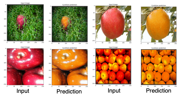
We can now forward pass our test inputs through our trained CycleGAN generator using the model.predict() function and save the outputs in preds, as shown on Line 45.

To visualize the predictions, we first use the matplotlib subplots to initialize subplots, as shown on Lines 49 and 50. Note that the subplot function takes as an argument the number of rows and columns and the size of the figure to be plotted, as shown.

We then instantiate a for loop to plot the results (Line 53). Next, we plot the input image by first converting the input (i.e., inp) to an image using the array_to_img() function (Line 56) and setting the image title to “Input Image” (Line 57). Then, we plot the corresponding CycleGAN output (i.e., pred) (Line 60) and set the image title to “CycleGAN prediction” (Line 61). Similarly, we plot the ground truth image (i.e., tar) (Lines 64 and 65).

Now that we have visualized our results, we check whether the output image directory where we will save our results exists, and if it does not, we create it (Lines 69 and 70).

Finally, we save our visualization using fig.savefig at the given path, which is config.GRID_IMAGE_PATH (Line 74).

---

---

Summary

In this tutorial, we continued our discussion on building an unpaired image translation model and looked into the training process of our CycleGAN pipeline.

Specifically, we developed our data pipeline and implemented the CycleGAN training pipeline from scratch in Keras and TensorFlow. Furthermore, we looked into the inference stage of our CycleGAN model and discussed how we can use the trained model for translating images from one domain to another in real-time.

---

Citation Information

Chandhok, S. “CycleGAN: Unpaired Image-to-Image Translation (Part 3),” PyImageSearch, P. Chugh, A. R. Gosthipaty, S. Huot, K. Kidriavsteva, R. Raha, and A. Thanki, eds., 2023, https://pyimg.co/b1qon

@incollection{Chandhok_2023_CycleGAN-Part3,
  author = {Shivam Chandhok},
  title = {{CycleGAN}: Unpaired Image-to-Image Translation (Part 3)},
  booktitle = {PyImageSearch},
  editor = {Puneet Chugh and Aritra Roy Gosthipaty and Susan Huot and Kseniia Kidriavsteva and Ritwik Raha and Abhishek Thanki},
  year = {2023},
  url = {https://pyimg.co/b1qon},
}

---

---

To download the source code to this post (and be notified when future tutorials are published here on PyImageSearch), simply enter your email address in the form below!

The post CycleGAN: Unpaired Image-to-Image Translation (Part 3) appeared first on PyImageSearch.