Statistical Experiments With Resampling

Bootstrapping and permutation tests

Introduction

Most people working with data make observations and then wonder whether these observations are statistically significant. And unless one has some formal training on statistical inference and past experience in running significance tests, the first thought that comes to mind is to find a statistician who can provide advice on how to conduct the test, or at least confirm that the test has been executed correctly and that the results are valid.

There are many reasons for this. For a start, it is often not immediately obvious which test is needed, which formulas underpin the test principles, how to use the formulas, and whether the test can be used in the first place, e.g. because the data do not fulfil necessary conditions such as normality. There are comprehensive R and Python packages for the estimation of a wealth of statistical models and for conducting statistical tests, such as statsmodels.

Still, without full appreciation of the statistical theory, using a package by replicating an example from the user guide often leaves a lingering sense of insecurity, in anticipation of severe criticism once the approach is scrutinised by a seasoned statistician. Personally, I am an engineer that turned into a data analyst over time. I had statistics courses during my undergraduate and postgraduate studies, but I did not use statistics extensively because this is not typically what an engineer does for a living. I believe the same applies to many other data analysts and data scientists, particularly if their formal training is for example in engineering, computer science or chemistry.

I decided to write this article because I came recently to the realisation that simulation can be readily used in place of more classical formula-based statistical methods. Most people would probably think immediately of bootstrapping to estimate the uncertainly of the mean. But it is not only about bootstrapping. Using resampling within random permutation tests can provide answers to many statistical inference problems. Such tests are generally not very difficult to write and execute. They apply universally to continuous or binary data, regardless of sample sizes and without making assumptions about the data distribution. In this sense, permutation tests are non-parametric and the only requirement is exchangeability, i.e. the probability to observe a certain sequence of values is the same for any permutation of the sequence. This is really not much to ask.

The unavailability of computing resources was perhaps one of the reasons for the impressive advancement of formula-based statistical inference tests in the past. Resampling thousands of times a data sample with tens or thousands of records was prohibitive back then, but it is not prohibitive anymore. Does this mean that classical statistical inference methods are not needed any more? Of course not. But having the ability to run a permutation test and confirm the results can be re-assuring when the results are similar, or help understand which assumptions do not hold when we observe discrepancies. Being able to run a statistical test from scratch without relying on a package also gives some sense of empowerment.

Permutation tests are of course nothing new, but I thought it is a good idea to provide some examples and the corresponding code. This may alleviate the fear of some data experts out there and bring statistical inference using simulation closer to their everyday practice. The article uses permutation tests for answering two questions. There are many more scenarios when a permutation test can be used and for more complex questions the design of a permutation test may not be immediately obvious. In this sense, this article is not comprehensive. However, the principles are the same. By understanding the basics it will be easier to look up an authoritative source on how to design a permutation test for answering other, more nuanced, business questions. My intention is to trigger a way of thinking where simulating the population distribution is at the centre and using the theoretical draws allows estimating what is the probability of an observed effect to occur by chance. This is what hypothesis tests are about.

Statistical inference starts with a hypothesis, e.g. a new drug is more effective against a given disease compared to the traditional treatment. Effectiveness could be measured by checking the reduction of a given blood index (continuous variable) or by counting the number of animals in which disease cannot be detected following treatment (discrete variable) when using the new drug and the traditional treatment (control). Such two-group comparisons, also known as A/B tests, are discussed extensively in all classical statistics texts and in popular tech blogs such as this one. Using the drug design example, we will test if the new drug is more effective compared to the traditional treatment (A/B testing). Building on this, we will estimate how many animals we need to establish that the new drug is more effective assuming that in reality it is 1% more effective (or for another effect size) than the traditional treatment. Although the two questions seem unrelated, they are not. We will be reusing code from the first to answer the second. All code can be found in my blog repository.

I welcome comments, but please be constructive. I do not pretend to be a statistician and my intention is to help others go through a similar learning process when it comes to permutation tests.

A/B testing

Let’s come back to the first question, i.e. whether the new drug is more effective than the traditional treatment. When we run an experiment, ill animals are assigned to two groups, depending on which treatment they receive. The animals are assigned to groups randomly and hence any observed difference in the treatment efficacy is because of drug effectiveness, or because it just happened by chance that the animals with the stronger immune system were assigned to the new drug group. These are the two situations that we need to untangle. In other words, we want to examine if random chance can explain any observed benefits in using the new drug.

Let’s come up with some imaginary numbers to make an illustration:

https://medium.com/media/0c4d8c5605b4b71904d9f231cf5f5fd6/href

The response variable is binary, i.e. the treatment was successful or not. The permutation test would work in the same way if the response variable was continuous (this is not the case with classical statistical tests!), but the table above would contain means and standard deviations instead of counts.

We intentionally do not use treatment groups of the same size, as this is not a requirement for the permutation test. This hypothetical A/B test involved a large number of animals and it seems that the new drug is promising. The new drug is 1.5% more effective than the traditional treatment. Given the large sample, this appears significant. We will come back to this. As humans, we tend to see as significant things that may not be. This is why standardising hypothesis tests is so important.

“Think about the null hypothesis as nothing has happened, i.e. chance can explain everything.”

In A/B testing, we use a baseline assumption that nothing special has been observed. This is also known as the null hypothesis. The person running the test usually hopes to prove that the null hypothesis does not hold, i.e. that a discovery has been made. In other words, the alternative hypothesis is true. One way of prove this is to show that random chance has a very low probability of leading to a difference as extreme as the observed one. We are already starting to see the connection with the permutation testing.

Imagine a procedure where all animals treated are pooled together into a single group (of 2487 + 1785 animals) and then split again randomly into two groups with the same sizes as two original treatment groups. For each animal we know if the treatment was successful or not and hence we can calculate the percentage of animals cured for each group. Using the observed data, we established that the new drug increased the percentage of cured animals from 80.34 to 81.79%, i.e. an increase of almost 1.5%. If we resample the two groups many times, how often would we see that the new drug leads to a greater percentage of animals being cured compared to the traditional treatment? This “how often” is the ubiquitous p-value in statistical inference. If it happens often, i.e. the p-value is larger than a threshold we are comfortable with (the also ubiquitous significance level, often 5%), then what we saw in the experiment can be due to chance and hence the null hypothesis is not rejected. If it happens rarely, then chance alone cannot lead to the observed difference and hence the null hypothesis is rejected (and you can organise a party if your team discovered the new drug!). If you observe carefully what we actually did with the permutations is to simulate the null hypothesis, i.e. that the two treatment groups are equivalent.

Think again about how the null hypothesis has been formulated, as this determines how the permutation testing will be conducted. In the example above, we want to see how often chance would make us believe that the alternative hypothesis is true, i.e. the new drug is more effective. This means that the null hypothesis, which is complementary to the alternative hypothesis, states that the new drug is less efficient or as efficient as the traditional treatment. This is also known as one-way test (vs. a two-way test, also known as a bi-directional test). Think of this in another way. We do not want to be fooled by random chance into believing that the new drug is more effective. Being fooled in the other direction does not matter, because we do not intend to replace the traditional treatment anyway. The two-way test would lead to higher p-values and is hence more conservative because it has a greater chance rejecting the null hypothesis. However, this does not mean that it should be used if it is not the right test to use.

The permutation test can be formulated in the most general case as follows. Let’s assume that there are Gᵢ, i=1,..,Nᴳ groups with cardinality ∣ Gᵢ ∣, i=1,..,Nᴳ:

• Pool together all data points from all groups; this essentially simulates the null hypothesis by assuming that nothing has happened.
• Randomly assign ∣ G₁ ∣ points to group G₁ without replacement, assign ∣ G₂ ∣ points to group G₂ without replacement, .., until all points have been assigned.
• Compute the statistic of interest as calculated in the original samples and record the result.
• Repeat the above procedure a large number of times and record each time the statistic of interest.

Essentially, the above procedure builds a distribution with the statistic of interest. The probability of observing a value that is at least as extreme as the observed difference is the p-value. If the p-value is large, then chance can easily produce the observed difference and we have not made any discovery (yet).

“Think about the p-value as being the probability of observing a result as extreme as our observation if the null hypothesis were true.”

The above formulation is quite generic. Coming back to our example, we only have two groups, one for the new drug and one for the traditional treatment. The code for carrying out the permutation test is below.

https://medium.com/media/b519772b9fe8eba4952d1db51bce0aa0/href

We do 10,000 permutations, which take approximately 30 seconds on my machine. The key question is: how often does chance makes the new drug 1.5% or more efficient than the traditional treatment? We can visualise the histogram of the simulated effectiveness differences and also compute the p-value as shown below.

https://medium.com/media/bcdc4d4bb008947facbdc1b115ac81be/href

This gives the following histogram:

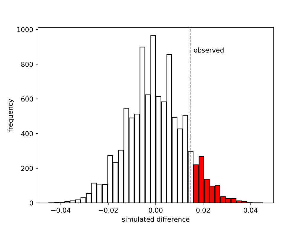
The red bars indicate when the new drug was found to be more effective than the traditional treatment by chance. This does not seem so rare. The p-value is 0.1084. Assuming that we wanted to run the test with a significance level of a=0.05, this means that the null hypothesis cannot be rejected. Nothing to celebrate at this point in time. If you have organised a party it needs to be cancelled. Or perhaps postponed.

“Think of a as the false positive rate, i.e. assuming that the null hypothesis is true we would conclude that there is a statistically significant difference in 5% of the time if we were to run the experiment repeatedly.”

There is some reason to be optimistic. The A/B test we just ran can have two possible outcomes: either there is an effect (in our case the new drug is more effective than the traditional treatment) or there is no sufficient evidence to conclude that there is an effect. The test does not conclude that there is no effect. The new drug could be more effective after all. We just cannot prove this yet at the chosen significance level with the data so far. The test has essentially protected us against a false positive (also known as a Type 1 error); but it could be that we have a false negative (also known as a Type 2 error). This is what the team hopes.

There is another question we could ask. What would the observed difference need to be to conclude that the new drug is more effective than the traditional treatment? Clearly 1.5% is not sufficient, but how much would be sufficient? The answer can be readily obtained from the produced histogram. We can “move” the vertical line corresponding to the observed difference to the right, until the tail with the red bars accounts for 5% of the total area; or in other words use the 95% percentile np.percentile(differences, 95), which gives 0.0203 or 2.03%. A bit more than the 1.5% we observed unfortunately, but not terribly off.

Using a significance level of 0.05, we would not reject the null hypothesis if the increase in the treatment effectiveness with the new drug is in the interval (-∞, 0.0203]. This is also known as the confidence interval: the set of values of the observed statistic that would not reject the null hypothesis. Because we used a 5% significance level this is a 95% confidence interval. Assuming that the new drug is not more efficient, then running the experiment multiple times would give a difference in effectiveness within the confidence interval 95% of the times. This is what the confidence interval tells us. The p-value will exceed a if and only if the confidence interval contains the observed effectiveness increase that means that the null hypothesis cannot be rejected. These two ways of checking whether the null hypothesis can be rejected are of course equivalent.

With the number of animals tested so far we cannot reject the null hypothesis, but we are not very far from the confidence interval bound. The team is optimistic, but we need to collect more compelling evidence that the new drug is more effective. But how much more evidence? We will revisit this in the next section, as running a simulation with resampling can help us answering this question too!

Before we conclude this section, it is important to note that we could also use a classical statistical test to approximate the p-value. The table presented above is also known as contingency table, which provides the interrelation between two variables and can be used to establish whether there is an interaction between them. The independence of the two variables can be examined using a chi-square test starting from the contingency matrix but care is needed not to run a two-sided test (did not try extensively, but scipy seems to use a two-sided as the default; this will lead to higher p-values). Isn’t it nice to know how to run a permutation test before delving into the user guide of statistical libraries?

Power estimation

Surely one would be disappointed given that we cannot prove that the increased effectiveness of the new drug is statistically significant. It could well be that the new drug is truly better after all. We are willing to do more work by treating more animals, but how many animals would we need? This is where power comes in.

Power is the probability of detecting a given effect size for a given sample size and level of significance. Let’s say that we expect the new drug to increase the treatment effectiveness by 1.5% compared to the traditional treatment. Assuming that we have treated 3000 animals with each treatment and fixed the level of significance to 0.05, the power of the test is 80%. This means that if we repeat the experiment many times we will see that in 4 out of 5 experiments we conclude that the new drug is more effective than the traditional treatment. In other words, the rate of false negatives (Type II error) is 20%. The numbers above are of course hypothetical. What is important is that the four quantities: sample size, effect size, level of significance and power are related and setting any three of them allows the fourth one to be computed. The most typical scenario is to compute the sample size from the other three. This is what we investigate in this section. As a simplification, we assume that in each experiment we treat the same number of animals with the new drug and the traditional treatment.

The procedure below attempts to construct a curve with the power as a function of the sample size:

• Create a synthetic dataset with animals supposed to have undergone the traditional treatment so that the treatment effectiveness is more or less what we know it to be (below, I set it to 0.8034 that corresponds to the contingency matrix above).
• Create a synthetic dataset with animals supposed to have undergone the treatment with the new drug by adding the effect size we would like to investigate (below, I set this to 0.015 and 0.020 to see its effect on the results).
• Draw a bootstrap sample of size n_sample from each synthetic dataset (below I set this to the values 3000, 4000, 5000, 6000 and 7000).
• Carry out a permutation test for statistical significance using the approach we established in the previous section and record whether the difference in treatment effectiveness is statistically significant or not.
• Keep generating bootstrap samples and compute how often the difference in treatment effectiveness is statistically significant; this is the power of the test.

This is of course a lengthier simulation and hence we limit the number of bootstrap samples to 200, whilst the number of permutations in the significance test is also reduced to 500 compared to the previous section.

https://medium.com/media/3533e1e224497a1caf6763acedcb08ab/href

Running this bootstrapping/permutation simulation takes an hour or so on a modest machine and could benefit from multiprocessing that is beyond the scope of this article. We can readily visualise the results using matplotlib:

https://medium.com/media/40160532c86be22789a356e8b390d211/href

This produces this graph:

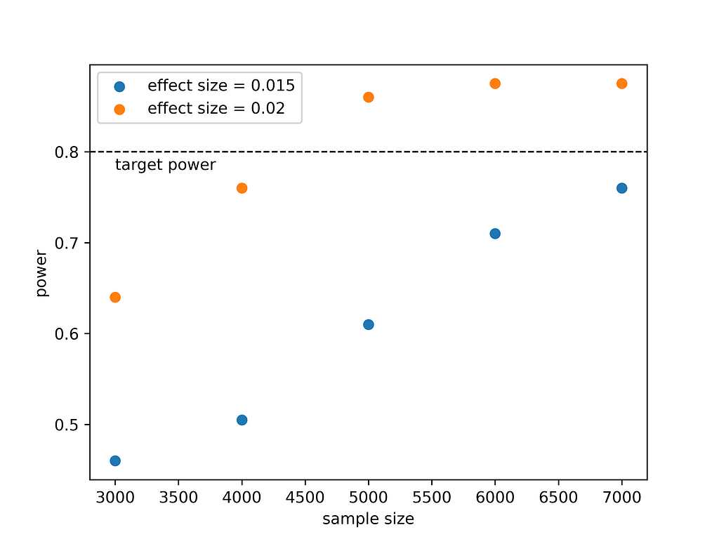
What do we learn from this? If we expect that the new drug is 1.5% more effective, then to prove this with a power of 80% we would need to treat more than 7000 animals. If the effect size is larger, i.e. 2%, we would need to work less as ~4500 animals would suffice. This is intuitive. It is easier to detect a large effect than a small effect. Deciding on running such a large experiment requires a cost/benefit analysis but at least now we know what it takes to prove that the new drug is more effective.

We can also use statsmodels to compute the required sample size:

https://medium.com/media/6a9e219009c366566290dcde139061ec/href

This prints:

effect size: 0.015, sample size: 8426.09
effect size: 0.020, sample size: 4690.38

The results from the simulation seem consistent. In the simulation we went up to a sample size of 7000 that was not sufficient to reach a power of 0.8 when the effect size was 1.5% as also seen using the proportion_effectsize function.

Concluding thoughts

I hope you enjoyed this article. Personally I find it fulfilling to be able to investigate all these statistical concepts from scratch using simple bootstrapping and permutations.

Before we close, a note of caution is due. This article puts much emphasis on the p-value that is increasingly being criticized. The truth is that the importance of the p-value has historically been exaggerated. The p-value indicates how incompatible the data are with a statistical model or permutation test representing the null hypothesis. The p-value is not the probability that the alternative hypothesis is true. Moreover, a p-value that shows that the null value can be rejected does not mean that the size of the effect is important. A small effect size may be statistically significant, but it is so small that this is not important.

References

• Introductory Statistics and Analytics: A Resampling Perspective by Peter Bruce (Wiley, 2014)
• Practical Statistics for Data Scientists: 50+ Essential Concepts Using R and Python by Peter Bruce, Andrew Bruce, Peter Gedeck (O’Reilly, 2020)
• Interpreting A/B test results: false positives and statistical significance, a Netflix technology blog

Statistical Experiments With Resampling was originally published in Towards Data Science on Medium, where people are continuing the conversation by highlighting and responding to this story.